Disclaimer: Please note that the information presented in this article is for informational purposes only. It is not intended to serve as health advice, engineering advice, or any form of professional guidance. Readers should consult with qualified professionals for specific health or engineering concerns and should not rely solely on the content of this article for making decisions. The authors and publishers of this article are not responsible for any actions taken based on the information provided herein. This article additionally covers a proof-of-concept bioreactor simulation. It is not a validated model of any real plant, and nothing here should be used to make process decisions.
My senior design project was 1,3-propanediol production from L. reuteri, so I thought some bioreactor modeling would be cool to do. I could not find a dataset online that fit the purpose. Then I found one for penicillin, and decided that if anything in fermentation was well modeled, penicillin probably was. Model predictive control (MPC) was interesting because it was a control scheme I was not familiar with.
Then it sat for a year while I was tied up elsewhere. I recently put the finishing touches on it, because a lengthy work engagement was coming and I wanted it out before then.
I cannot put hours on any of this. I picked at it casually, alongside other projects, while working through my master’s degree. Learning Rust helped dramatically. The work itself was no easier or harder in either language. It all sucked. The draw of Rust was that I could easily export it to WASM and run it on the web, where before I was constrained to Python with no clean, fast way of sharing the result. The draw of Python was being able to back-check the mathematics there before I moved to Rust. Being able to share things online definitely helps my motivation.
The tool is a fed-batch penicillin fermenter that runs in the browser under three controllers at once: PID, MPC, and PID with an MPC correction on top. Fed-batch means the tank is fed sugar continuously while the batch runs, instead of being given all of it at the start. The physics and the optimizer are Rust compiled to WebAssembly. It is live at bioreactor-mpc.jesse-anderson.net.
This post is mostly about the model underneath the controllers, and how far it can be trusted.
The model is the five differential equations of Bajpai and Reuss (1980). I tested it against IndPenSim, a published simulator of a 100,000 L industrial penicillin fermenter that ships with 100 recorded batches. Its authors built it as a mechanistic model and validated it against records from ten real batches. So “ground truth” here means a far more detailed model, and the comparison is one model against another: a small one from 1980 and a large one from 2015.
Table of Contents
The Short Version
- The paper’s parameters make about 1 g/L of penicillin. The plant makes 30. Nothing replays until you refit.
- After refitting twelve constants on six batches, the model tracks penicillin on the 44 held-out normal batches with a median R² of 0.987.
- In 48 of the 100 batches the recorded sugar builds up, which the model cannot reproduce. In 42 of those 48 the cause is a single switch in IndPenSim that my model has no state for.
- Two of the twelve fitted constants finished pinned at their lower bounds, the aeration exponent and the Contois constant for sugar. Both wanted to go further, and each one explains a specific thing the model gets wrong.
- A proper refit, run for this post, fixes the sugar level and leaves the 48 batches exactly where they were.
Everything below is the why, plus the parts that went wrong.
1. The Model
The model tracks five quantities in the tank, called states, and is driven by two inputs.
| Symbol | What it is | Unit |
|---|---|---|
| \(X\) | Biomass: the dry weight of cells per liter of broth | g/L |
| \(P\) | Penicillin concentration | g/L |
| \(S\) | Substrate: the sugar the cells eat | g/L |
| \(C_L\) | Oxygen dissolved in the broth | mmol/L |
| \(V\) | Broth volume | L |
| \(F\) | Input: the feed rate of sugar solution | L/h |
| \(K_La\) | Input: the oxygen transfer coefficient | 1/h |
\(K_La\) is one number, written as a product by convention. It says how fast oxygen moves from the air bubbles into the liquid, and it stands in for everything the plant does to move it: aeration and agitation.
Each state has a differential equation, which gives the rate at which that state is changing right now. The simulator steps those rates forward in time. Two of the rates come first, because the balances are built from them.
Growth. The specific growth rate \(\mu\) is how fast the cells multiply, per gram of cells. It follows Contois kinetics in both sugar and oxygen. Contois is a saturation law: growth rises with the nutrient and levels off, and the level at which it reaches half of its maximum scales with biomass. So a dense culture grows more slowly on the same sugar.
\[ \mu = \mu_x \,\frac{S}{K_x X + S}\,\frac{C_L}{K_{ox} X + C_L} \]
Where:
- \(\mu\) is the specific growth rate in 1/h: grams of new cells per gram of cells per hour.
- \(\mu_x\) is the largest value \(\mu\) can take, when neither sugar nor oxygen is limiting.
- \(K_x\) is the Contois constant for sugar, in grams of sugar per gram of cells. The sugar fraction is one half when \(S = K_x X\).
- \(K_{ox}\) is the same constant for oxygen, in mmol of oxygen per gram of cells.
- \(X\), \(S\), and \(C_L\) are the states from the table above.
Each fraction runs from 0 to 1. With plenty of sugar and oxygen both are close to 1 and \(\mu\) is close to \(\mu_x\). If either nutrient runs out, its fraction goes to 0 and takes growth with it.
Production. The specific production rate \(\mu_{pp}\) is how fast the cells make penicillin, per gram of cells. It has a substrate-inhibition term in sugar, so it rises with sugar and then falls.
\[ \mu_{pp} = \mu_p \,\frac{S}{K_p + S + S^2/K_I}\,\frac{C_L^{\,p}}{K_{op} X + C_L^{\,p}} \]
Where:
- \(\mu_{pp}\) is the specific production rate in 1/h: grams of penicillin per gram of cells per hour.
- \(\mu_p\) is its ceiling. The sugar fraction below can never quite reach 1, so the real maximum is a little under \(\mu_p\).
- \(K_p\) is the saturation constant for sugar, in g/L. It sets how much sugar production needs before it gets going.
- \(K_I\) is the inhibition constant, in g/L. It sets how much sugar it takes to shut production down again.
- \(K_{op}\) is the oxygen constant for production, and \(p\) is an exponent, 2.74 in the paper, that makes production more sensitive to low oxygen than growth is.
The \(S^2/K_I\) term is why a penicillin fermentation is run the way it is. With too little sugar the cells have nothing to make product from, and with too much, production switches off. The maximum sits at \(S = \sqrt{K_p K_I}\), which with the paper’s constants is 4.5 mg/L.
Worked with the paper’s constants and oxygen not limiting, the sugar fraction as a share of its own maximum:
| Sugar in the broth | Production, share of maximum |
|---|---|
| 0.1 mg/L | 36% |
| 1 mg/L | 90% |
| 4.5 mg/L | 100% |
| 20 mg/L | 90% |
| 100 mg/L | 54% |
| 1 g/L | 10% |
| 10 g/L | 1% |
A batch starts with grams of sugar per liter so the cells can grow, and is then held at a few milligrams per liter so they produce. The reactor is run nearly starved for more than a week.
The authors say plainly where that term comes from. They could not find a biochemical mechanism in the literature, chose the inhibition form because it reproduces the behavior, and warn that its success “should not be considered to throw any light upon the nature of phenomena involved”.
The balances. Each one says that a state changes by what is made, minus what is used up, plus what flows in, minus what is diluted away.
\[ \begin{aligned} \frac{dX}{dt} &= \underbrace{\mu X}_{\text{growth}} - \underbrace{\frac{F}{V}X}_{\text{dilution}} \\[6pt] \frac{dP}{dt} &= \underbrace{\mu_{pp} X}_{\text{production}} - \underbrace{K_d P}_{\text{hydrolysis}} - \underbrace{\frac{F}{V}P}_{\text{dilution}} \\[6pt] \frac{dS}{dt} &= -\underbrace{\frac{\mu X}{Y_{x/s}}}_{\text{eaten for growth}} - \underbrace{\frac{\mu_{pp} X}{Y_{p/s}}}_{\text{eaten for product}} - \underbrace{m_x X\,\frac{S}{k_{ms} + S}}_{\text{maintenance}} + \underbrace{\frac{F}{V}\,(S_f - S)}_{\text{feed}} \\[6pt] \frac{dC_L}{dt} &= -\underbrace{\frac{\mu X}{Y_{x/o}}}_{\text{growth}} - \underbrace{\frac{\mu_{pp} X}{Y_{p/o}}}_{\text{product}} - \underbrace{m_o X\,\frac{S}{k_{ms} + S}\,\frac{C_L}{K_{ox} X + C_L}}_{\text{maintenance}} + \underbrace{K_La\,(C_L^{*} - C_L)}_{\text{transfer from the air}} - \underbrace{\frac{F}{V}C_L}_{\text{dilution}} \\[6pt] \frac{dV}{dt} &= \underbrace{F}_{\text{feed}} \end{aligned} \]
Where:
- \(F/V\) is the dilution rate in 1/h. Feed adds volume, and every concentration in the tank is thinned by it.
- \(K_d\) is the hydrolysis constant in 1/h. Penicillin breaks down in water, a fixed fraction per hour.
- \(Y_{x/s}\) and \(Y_{p/s}\) are yields on sugar: grams of cells, or of penicillin, made per gram of sugar eaten. Dividing by a yield turns a rate of making into a rate of eating.
- \(Y_{x/o}\) and \(Y_{p/o}\) are the same yields on oxygen, per mmol of oxygen.
- \(m_x\) and \(m_o\) are maintenance coefficients: the sugar (g per gram of cells per hour) and oxygen (mmol per gram of cells per hour) that cells burn just to stay alive, growing or not.
- \(k_{ms}\) is a small sugar concentration, in g/L, below which maintenance fades out. It is my addition and is explained next.
- \(S_f\) is the sugar concentration of the feed, in g/L.
- \(C_L^{*}\) is the oxygen saturation, in mmol/L: the most oxygen the broth can hold at the current pressure. Oxygen moves in faster the further \(C_L\) is below it.
Two things here are my additions to the paper.
The maintenance gate. In the paper, maintenance is a flat \(m_x X\) drawn from the sugar and \(m_o X\) from the oxygen. A flat draw keeps drawing when the tank is empty, and \(S\) goes negative. The usual fix is to clamp the state. Here maintenance fades out through \(S/(k_{ms}+S)\) with \(k_{ms} = 10^{-4}\) g/L, which keeps sugar and oxygen non-negative without clamping the state.
The reason is the operating point. A penicillin batch sits at a few milligrams of sugar per liter for 200 hours, so the model spends most of its time close to zero sugar. The MPC needs the model’s Jacobian, the matrix of how each rate responds to a small change in each state. It gets one every three minutes by nudging each state slightly and differencing the results, which is a finite-difference Jacobian. A clamp puts a corner in the right-hand side at exactly that point, and a finite difference taken across a corner is wrong on both sides of it. The gate is smooth. With it, every term that consumes sugar or oxygen goes to zero as that resource does, so the states stay non-negative by construction. The integrator, the linearization, and the Python reference all inherit that without each needing its own identical clamp.
The gate has two costs. This process runs at a few milligrams of sugar per liter, which is close to \(k_{ms}\), so the gate changes the maintenance term at the operating point. At 10 mg/L it passes 99% of the paper’s maintenance, and at 1 mg/L it passes 91%. It also adds a steep slope of its own to the sugar balance, \(m_x X / k_{ms}\), which is most of that balance’s stiffness.
Substepped RK4. The simulator steps the equations forward with RK4, the classic fourth-order Runge-Kutta method, on a fixed step of 0.01 h. The oxygen balance is stiff, meaning it reacts far faster than everything else in the model, and a fixed-step method goes unstable when its step is too long for the fastest thing in the system. When the culture is oxygen-limited the uptake term has a slope of \((\mu_x/Y_{x/o} + m_o)/K_{ox}\), which with the paper’s numbers is about \(10^4\) per hour. A fixed-step RK4 at 0.01 h is far outside its stability region there and diverges. The sugar balance is stiff too, in the low thousands per hour at production biomass. At each step the integrator computes a worst-case rate over both balances and subdivides the step until it is stable.
Bajpai and Reuss had the same problem. Their first integrator, a predictor-corrector without step-size control, “was found to result in instabilities even for a case of no oxygen limitation”, and they switched to a semi-implicit Runge-Kutta method. On an HP 3000, 150 hours of fermentation took 15 to 20 seconds of processor time. They name the same two trouble spots, dissolved oxygen at high growth rates and penicillin production at low sugar. So the stiffness comes from the equations themselves.
For replaying plant data the model also takes three exogenous inputs: substrate-free liquid in (\(F_{dil}\): water, acid, base, and precursor, minus evaporation), broth out (\(F_{out}\)), and a time-varying oxygen saturation. With all three at zero it is exactly the equations above.
2. The Paper Makes 1 g/L. The Plant Makes 30.
The paper’s parameters describe a laboratory strain on synthetic medium, estimated from batch data already in the literature. Its figures report penicillin as activity, on axes that top out between 1400 and 3000 U/cm³. At 0.6 µg per unit that is 0.8 to 1.8 g/L. My lab-scale scenario, on the same parameters, reaches about 0.6 g/L in 100 hours. The IndPenSim batches end around 30 g/L.
Tuning cannot close that gap. Decades of strain improvement separate the two numbers, and no input schedule gets the paper’s kinetics to 30 g/L. The authors expected as much. They wrote that the parameters “are likely to be a strong function of the strain and its morphology” and that “no attempt was made to estimate an exact set”. For the oxygen-limited model, the abstract claims that observed trends “have been predicted qualitatively”. The paper offers a structure and expects you to refit it.
So there are two parameter sets. The paper’s set is untouched and is still the default. A second, plant-scale set is fitted to IndPenSim. The fitted values below are rounded to two figures.
| Constant | Paper | Fitted to IndPenSim | |
|---|---|---|---|
| \(\mu_x\) (1/h) | 0.092 | 0.18 | |
| \(K_x\) | 0.15 | 0.005 | at its lower bound |
| \(\mu_p\) (1/h) | 0.005 | 0.037 | 7× |
| \(K_p\) (g/L) | 0.0002 | 0.0018 | |
| \(K_I\) (g/L) | 0.1 | 0.0099 | |
| \(K_d\) (1/h) | 0.04 | 0.0081 | |
| \(Y_{x/s}\) | 0.45 | 0.40 | |
| \(m_x\) | 0.014 | 0.0085 | |
| \(S_f\) (g/L) | 50 | 600 | my choice at lab scale (the paper gives none); the plant’s value |
| \(C_L^{*}\) (mmol/L) | 0.25 | 0.52 | my choice at lab scale; from head pressure at plant scale |
Eight kinetic constants are fitted, plus four that map plant measurements onto model inputs. The oxygen yields stay at the paper’s values, because dissolved oxygen only identifies the ratio of uptake to transfer. The two oxygen constants, \(K_{ox}\) and \(K_{op}\), follow the paper’s own rules, re-evaluated at the new \(C_L^{*}\).
\(K_p\) and \(K_I\) moved in opposite directions. \(K_p\) went up ninefold and \(K_I\) went down tenfold, so their product barely moved. The production optimum \(\sqrt{K_p K_I}\) is 4.5 mg/L with the paper’s constants and 4.2 mg/L with the fitted ones. It looks as if the fit raised the production rate sevenfold and left the operating sugar level where the 1980 paper put it. That turns out to be an artifact of one bound, which section 8 takes apart.
Mapping a Plant Onto Two Inputs
Each IndPenSim row has 33 process columns ahead of the Raman spectrum. My model has two inputs. The mapping between them involves several judgment calls.
- Feed. IndPenSim feeds sugar and soybean oil. Both are carbon. I fold the oil into one sugar-equivalent feed, \(F = F_s + (C_{oil}/C_s)\,F_{oil}\), and take the volume the oil did not add back out through \(F_{dil}\).
- Oxygen transfer. \(K_La = k_0\,(F_g/60)^{\alpha}\).
- Oxygen saturation. \(C_L^{*} = h\,(p + p_0)\).
- Volume. Water, acid, base, and precursor dilute. Dumps remove broth. Evaporation is one constant, fitted to the volume balance alone.
Where:
- \(F_s\) and \(F_{oil}\) are the recorded sugar and oil feed rates, in L/h.
- \(C_s\) and \(C_{oil}\) are the substrate concentrations IndPenSim assigns to each feed, 600 and 1000 g/L. Their ratio converts a liter of oil into the liters of sugar feed that would carry the same substrate.
- \(F_{dil}\) is everything that adds volume without adding sugar: water, acid, base, and precursor, minus evaporation.
- \(F_g\) is the recorded aeration rate. Dividing by 60 makes the bracket equal to 1 at a typical mid-batch value.
- \(k_0\) is the fitted \(K_La\) at that reference aeration, and \(\alpha\) is the fitted exponent that says how strongly \(K_La\) responds to more air.
- \(p\) is the recorded head pressure in bar. \(h\) and \(p_0\) are fitted. \(p_0\) stands for the pressure the broth feels on top of the headspace, from the atmosphere and the depth of liquid.
3. Trusting the Model Before Trusting the Fit
A project like this can be wrong in three places, and each needs a different check.
Is the Rust the same as the Python? Every Rust component has a Python reference. The Python writes fixtures, which are files of inputs with the outputs it computed for them, and the Rust tests have to reproduce those outputs. The fixtures cover the rates, the Jacobians, single RK4 steps, the matrices of the MPC’s optimization problem, closed-loop runs with a controller in charge, and a 20-hour plant replay.
Is the Python the same as the paper? Those fixtures only prove that two implementations agree. If I transcribed a kinetic term wrongly, both would be wrong together and every test would pass.
This happened. For a while the Rust matched the Python exactly and the Python did not match the paper, with penicillin stuck near zero. The cause was the oxygen term and its constants. It hid until I went back and began tinkering with the equations one night after dying in Bloodborne(I was pissed and moved from one failed hard task to another).
So a separate script now runs the Python model against the paper’s own figures. This check is weaker than I would like. The paper states its feed as grams of glucose per liter of broth per hour and never gives a feed concentration. For the two fitted experiments the initial biomass has to be read off a figure.
Penicillin is reported as activity, and the only conversion in the text is an aside equating a production rate of “5 U g⁻¹ h⁻¹” with 0.003 1/h. Taken literally that is 0.6 mg per unit, which would put the paper’s own figures at hundreds of grams per liter. Read per milligram of cells it gives 0.6 µg per unit, which is the standard penicillin unit and the only reading that makes physical sense, so that is the one I used. The comparison therefore covers trends and order of magnitude only.
Within those limits it passes. Penicillin after 100 hours rises with \(K_La\), collapses toward zero at low but finite \(K_La\), and levels off at high \(K_La\), as in the paper’s Figure 3. There is an interior optimum feed rate, as in Figure 4. The plateau in my Figure 3 run is 0.80 g/L, about 1340 U/cm³, on a figure whose axis ends at 2000. The best case in my Figure 4 run is 1.24 g/L, about 2070 U/cm³, on an axis that ends at 3000.
Is the model the same as the plant? That is the rest of this post.
4. What Twelve Fitted Constants Bought
The Dataset
IndPenSim’s public dataset is 100 simulated batches. Each runs for roughly 230 hours and is sampled every 12 minutes. The dataset groups them by how the batch was run:
| Batches | Regime | What it means |
|---|---|---|
| 1 to 30 | Recipe-driven | Feeds follow a fixed schedule. |
| 31 to 60 | Operator-controlled | A simulated operator adjusts that schedule during the batch. |
| 61 to 90 | Advanced control | A controller manages the batch using a simulated Raman probe. Section 5 comes back to what it controls. |
| 91 to 100 | Faults | A fault is injected on purpose. |
Most signals are recorded at every sample. Biomass and a few others are only measured offline, from a sample taken about every 12 hours.
I split the batches two more ways for scoring.
- A batch has substrate accumulation if its recorded sugar goes above 1 g/L after penicillin has reached 1 g/L. That should never happen in a healthy batch, and section 5 is about why it does.
- A batch is normal if it has no accumulation and no injected fault.
The Fit and the Replay
The fit used six batches: 1, 2, 31, 32, 61, and 62, two from each of the first three regimes. These are the training batches. The other 94 never touched the optimizer, so they are held out: the model is scored on data it was not fitted to.
The replay is open loop. The model is given a batch’s recorded feeds, aeration, additions, dumps, and head pressure, and its outputs are compared with what was recorded. No controller is involved, and nothing corrects the model along the way.
Two scores appear from here on.
- RMSE is the root-mean-square error between the model and the recording, in the signal’s own units. Smaller is better.
- R² is one minus the ratio of the model’s squared error to the variance of the recording. A value of 1 is a perfect match, 0 is no better than predicting the recording’s average, and a negative value is worse than that.
Median scores over each group, whole batch:
| Group | Batches | Penicillin RMSE (g/L) | Penicillin R² | Biomass R² | Substrate R² | Oxygen R² | Volume R² |
|---|---|---|---|---|---|---|---|
| Training | 6 | 1.12 | 0.988 | 0.906 | 0.949 | 0.389 | 0.980 |
| Recipe-driven, normal | 15 | 1.25 | 0.987 | 0.952 | 0.936 | 0.336 | 0.979 |
| Operator-controlled, normal | 3 | 1.05 | 0.988 | 0.966 | 0.938 | 0.536 | 0.985 |
| Advanced control, normal | 26 | 1.16 | 0.987 | 0.953 | 0.960 | 0.407 | 0.980 |
| Substrate accumulation | 40 | 4.45 | 0.751 | 0.879 | -0.217 | -0.237 | 0.978 |
| Process faults | 10 | 8.38 | -4.238 | 0.742 | -0.491 | -0.662 | 0.978 |
The accumulation row holds the 40 such batches that have no injected fault. The other 8 accumulating batches are fault batches and are counted in the last row, which is why this table says 40 where section 5 says 48.
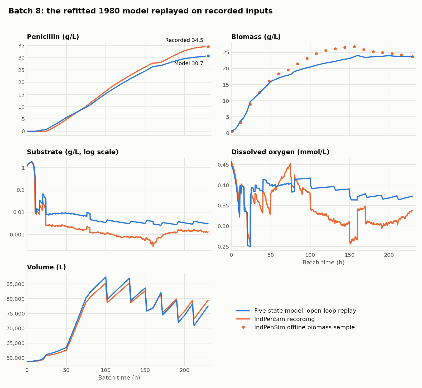
Held-out batches score the same as the training batches. Across the 44 held-out normal batches the median penicillin R² is 0.987 with an RMSE of 1.2 g/L on a signal that ends near 30.
R² on a curve like this is forgiving, so I also checked the end point. Across those 44 batches the model’s final penicillin is off by a median of +0.3 g/L, with half of them inside -1.0 to +1.6 and the worst at -3.8 and +5.1.
That result is easier to get than it sounds. Penicillin in a healthy batch is a smooth curve that rises for 200 hours, and twelve free constants with the recorded inputs should be able to follow it. It shows that the structure of the 1980 model is enough for a healthy batch, and it says nothing about an unhealthy one.
5. Forty-Eight Batches the Model Cannot See
In 48 of the 100 batches the recorded substrate climbs above 1 g/L during production, three orders of magnitude above where it should be. In 43 of them it passes 5 g/L and penicillin stops rising and falls. The median batch among those loses 36% of its peak by the end. My model keeps producing through all of it.
The size of the miss, over those 43:
| Recorded | Model | |
|---|---|---|
| Median final penicillin, collapsing batches | 16.0 g/L | 31.6 g/L |
| Median final penicillin, all other batches | 30.4 g/L | 30.7 g/L |
My first assumption was that the mistake was mine. I always assume I am wrong and stupid, which is a safer bet than blindly trusting an output. I had reason to here. For the longest time I could not get these equations to converge in Python, so I suspected my mathematics before I suspected anything else.
My previous README’s note on this was “the model has no mechanism for that”. That is true and explains nothing, so I looked for the mechanism.
Accumulation Follows the Control Strategy
| Regime | Batches | Accumulate |
|---|---|---|
| Recipe-driven (1-30) | 30 | 13 |
| Operator-controlled (31-60) | 30 | 25 |
| Advanced control (61-90) | 30 | 2 |
| Faults (91-100) | 10 | 8 |
Twenty-five of the thirty operator-controlled batches accumulate, against two of the thirty under advanced control. Whatever causes this, the control strategy decides whether it happens.
pH, Temperature, and Oxygen Do Not Explain It
Around the penicillin peak in the 35 collapsing batches without injected faults, taking medians twelve hours before, two hours before, and six hours after:
| Signal | 12 h before | 2 h before | 6 h after |
|---|---|---|---|
| pH | 6.500 | 6.497 | 6.506 |
| Temperature (K) | 297.95 | 297.97 | 297.92 |
| Dissolved oxygen (mg/L) | 11.8 | 12.0 | 13.1 |
| Oxygen uptake rate | 1.37 | 1.33 | 0.89 |
pH and temperature do not move. Dissolved oxygen rises afterwards and oxygen uptake falls by a third, which is what cells do when they stop consuming. None of these signals changes before the peak.
The Precursor
Penicillin G is built from a core the cells make and a side chain they do not. The side chain is fed separately as phenylacetic acid (PAA), which is called the precursor. PAA is toxic to the same cells in excess. IndPenSim records its concentration offline, every twelve hours.
For each of the 90 batches without injected faults, I checked whether any offline PAA sample reached 2400 mg/L.
| PAA never sampled at 2400 mg/L | PAA sampled at 2400 mg/L or more | |
|---|---|---|
| No accumulation | 50 | 0 |
| Accumulation | 3 | 37 |
No batch sampled at 2400 mg/L or above stayed healthy.
By regime, the number of batches that ever sample PAA at 2400 mg/L or above is 12 of 30 recipe-driven, 25 of 30 operator-controlled, and 0 of 30 under advanced control. The highest PAA sample in any advanced-control batch is 1608 mg/L.
That table alone does not establish cause. Once production stops, the precursor stops being consumed and piles up, so a high sample after a collapse can be a consequence of it. The order of events has to be checked.
Offline samples are twelve hours apart, which is too coarse to see a crossing directly. So for each collapsing batch I took the last two PAA samples before the sugar leaves its production window, which I take as the last moment it is below 10 mg/L. I drew a line through those two samples and read off where PAA was at that moment.
| Extrapolated PAA when sugar leaves the window (mg/L) | |
|---|---|
| 35 collapsing batches without faults, median | 2392 |
| Middle half | 2360 to 2422 |
| Full range | 2297 to 2613 |
These 35 batches turn anywhere from 119 to 230 hours, and in 33 of them the precursor is within 5% of 2400 at that moment. The two outliers, batches 36 and 47, are ones where the last sample is 8 and 11 hours before the turn and the line through it is steep. Moving the edge of the window to 5, 10, or 50 mg/L of sugar leaves the median at 2392 or 2393.
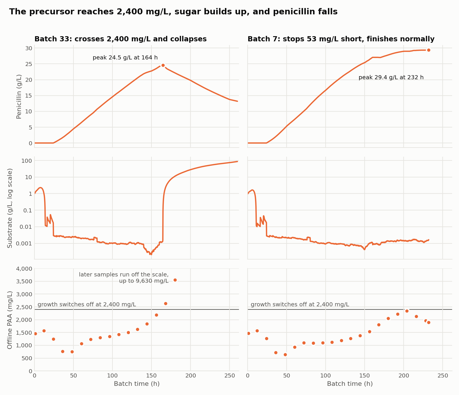
Batch 7 is a useful counter-case. Its PAA samples climb 1805, 2051, 2224, 2347, and then fall back to 2128 and 1962. It came within 53 mg/L of 2400 and finished normally at 29.4 g/L.
Then I Read the Source
The 2015 paper that introduces IndPenSim describes the mechanism. It says that high levels of PAA “are toxic to the biomass by inhibiting growth and penicillin production”, that the plant held PAA between 200 and 2000 mg/L, and that PAA flow “was manually adjusted based on off-line measurements of its concentration”, which were taken every 12 hours. The model has an inhibition term, written as a hyperbolic tangent, that takes the growth rate to effectively zero above a critical concentration.
The paper’s parameter table puts that critical concentration at 2000 mg/L. The recorded batches do not agree with 2000. Eight batches that never accumulate have samples above it, and batch 7 reaches 2347. The code released with the dataset has a different number. The default run script sets the inhibition flag to its full mode, which includes PAA. Parameter_list.m:
and indpensim_ode.m, where y(30) is the PAA concentration:
PAA_inhib_X = 0.5*(1+(tanh((X_crit_PAA - y(30)))));
...
mu_e = mux_max*pH_inhib*NH3_inhib*T_inhib*DO_2_inhib_X*CO2_inhib*PAA_inhib_X;
Where:
X_crit_PAAis the critical PAA concentration for growth.PAA_inhib_Xis a multiplier between 0 and 1 that is applied to growth.mu_eis one of IndPenSim’s two growth rates, the one for the extending tips of the fungus. The other one carries the same multiplier.mux_maxis the maximum growth rate, and the other_inhibnames are multipliers of the same kind for pH, nitrogen, temperature, dissolved oxygen, and carbon dioxide.
So the dataset was generated with 2400, where the paper says 2000, and the extrapolated median of 2392 from the data is consistent with the code. The term itself is a hyperbolic tangent with a slope of one per mg/L on a quantity in the thousands. It is a switch. At 2395 mg/L the cells grow normally, and at 2405 they do not grow at all.
The rest follows from a second line:
Here s is the substrate concentration in g/L and P_inhib is a multiplier on penicillin production. With mean_P = 0.002 and P_std_dev = 0.0015, that is a Gaussian, a bell curve, in substrate. Production runs at full rate at 2 mg/L of sugar and is effectively zero by 10 mg/L. The chain is:
- PAA crosses 2400 mg/L.
- Growth switches off, and the sugar the cells were taking up for growth stops being taken up.
- The feed keeps coming, so sugar accumulates.
- Sugar leaves the narrow window where penicillin is made.
- Production stops while hydrolysis and dilution continue, so penicillin falls.
Once growth and production stop, the two main sinks for the precursor stop with them, so PAA runs away. Later samples in these batches reach as high as 11,500 mg/L.
What the Model Is Missing
My model already has step 4. Its substrate-inhibition term does the same job as IndPenSim’s Gaussian: at 1 g/L of sugar, with the fitted constants, production is under 2% of its maximum. If sugar accumulated in my model, penicillin would stop.
Sugar never accumulates in my model, because its cells never stop growing. What it lacks is the trigger, which would take a sixth state for PAA and one switch on the growth rate.
The two models also agree on where the reactor should sit. IndPenSim centers production at 2 mg/L of sugar. The 1980 paper puts it at 4.5 and my fit at 4.2. In the healthy batches the recorded sugar during production has a median of 1.2 mg/L, and my replay of the same batches holds 3.8. Each model sits just under its own optimum.
The Six That Are Different
Six of the 48 have a different cause.
Three oxygen blips. Batches 27, 68, and 70 are flagged as accumulation and never go near 2400 mg/L. Around 90 hours dissolved oxygen dips below 3 mg/L, sugar blips to between 1.7 and 3.7 g/L, and then everything recovers. They finish at 27 to 30 g/L. Eleven batches show that same oxygen dip near 90 hours. Seven of them pass the 1 g/L line I used as a flag. Four of those seven go on to cross 2400 mg/L later and collapse for the usual reason. In these three the dip is the only thing that happened.
Three aeration faults. All eight accumulating fault batches have a PAA sample above 2400 mg/L, which is why the order of events matters. Five of them (91, 92, 95, 96, 97) extrapolate to between 2358 and 2447 mg/L at the turn, the same as the rest. The other three (94, 99, 100) are at 1800 to 2030. They are the only batches in the dataset where aeration is cut to 20. The cut from 75 lands at hour 100, and their sugar leaves the window at hour 100. PAA crosses afterwards, as a consequence. The 2019 paper lists its aeration faults at hours 20 to 24 and 100 to 110, which is where these sit.
That makes the count 42 of 48: the 37 without faults, and five with. Two of the 37, batches 46 and 48, only begin to turn in the last three hours of the batch, so they pass 1 g/L and never 5.
What This Shows
This explains why the model fails on these batches, and for 42 of them the failure has one cause. It is a statement about the benchmark, and the 2019 paper that released the dataset says as much. The existing strategy tries to hold PAA between 600 and 1800 mg/L by adjusting its feed. With a sample every 12 hours and a 4-hour delay on the assay, the paper says, “the control of this CPP remains suboptimal”. CPP a is critical process parameter, a variable that has to stay in range for the batch to meet its target.
The advanced-control batches are the paper’s answer. Raman spectroscopy reads the chemical makeup of the broth from scattered laser light, continuously and without taking a sample. A soft sensor, which is a statistical model that turns those spectra into a concentration, predicts PAA in real time. A PI loop, a PID controller without the derivative term, then adjusts the PAA feed to hold it at a setpoint of 1250 mg/L. In the recorded data no advanced-control batch samples PAA above 1608 mg/L, and the paper reports a 20% increase in annual penicillin yield for that campaign.
The operators here are simulated. The 2015 paper does say that on the real plant PAA was dosed by hand from the twelve-hourly samples, so the benchmark is imitating a real difficulty.
6. Two Constants Pinned at Their Floors
Dissolved oxygen is the weak signal even on healthy batches, with a median R² of 0.36 across the 44 held-out normal ones.
Two of the twelve fitted constants finished at their lower bounds. A constant stuck at a bound is one the fit wanted to push further than I let it. So I moved each one past its bound, with everything else held where the fit left it, and watched the fit’s own objective. The objective is the single number the fit minimizes: a weighted sum of the squared errors on penicillin, biomass, dissolved oxygen, and sugar over the six training batches. Lower is better, and the saved fit scores 298.
The aeration exponent. The mapping is \(K_La = k_0 (F_g/60)^{\alpha}\), and \(\alpha\) went to its floor of 0.01. At 0.01, \(K_La\) is effectively constant. Across the whole range of aeration in the dataset it moves by a little over 1%.
| \(\alpha\) | -1.0 | -0.5 | -0.25 | 0.01 (fit) | 0.25 | 0.5 |
|---|---|---|---|---|---|---|
| Objective | 323 | 275 | 278 | 298 | 331 | 380 |
The fit wanted a negative exponent. More air, less oxygen transfer. That is physically backwards, and IndPenSim’s own formula explains it. Its transfer coefficient goes as gas velocity to the power 0.38 and as viscosity to the power -0.38, both from the 2015 paper’s parameter table. The recipe steps aeration up through most of the batch, from 30 to 75, while the broth thickens from 4 cP to nearly 80. A centipoise (cP) is the unit of viscosity, and water is 1. My mapping has aeration and no viscosity, so its one exponent was absorbing both effects. Agitator speed carries no information, because it is 100 rpm in every row of every batch. The paper says the plant ran at a fixed 100 rpm.
The 1980 paper anticipated this. It notes that in mold fermentations \(K_La\) “drops significantly during the course of fermentation as a result of growth”, and that the authors “decided not to incorporate this factor”. My model inherits that decision, and Figure 1 shows the cost: after 100 hours the model’s dissolved oxygen stays near 0.38 mmol/L while the recording drops to about 0.31. The fix is a viscosity term. Allowing a negative exponent would improve the score without meaning anything physically.
The Contois constant. \(K_x\) went to its floor of 0.005.
| \(K_x\) | 0.001 | 0.0016 | 0.0025 | 0.005 (fit) | 0.01 |
|---|---|---|---|---|---|
| Objective | 345 | 255 | 241 | 298 | 457 |
| Model sugar in production (mg/L) | 1.1 | 1.5 | 2.1 | 3.8 | 7.7 |
\(K_x\) sets how low the cells can pull the sugar, and the recorded level on these batches is 1.25 mg/L. Halving the floor would have cut the objective by 19% and brought the model’s sugar level most of the way down.
I went back through the code for a numerical reason behind 0.005 and did not find one. A smaller \(K_x\) does steepen the sugar balance, from 88 per hour at 0.005 to 176 at 0.0025, but the oxygen balance is already at 8,300 and sets the substep count on its own. The finite-difference step in the linearization is \(10^{-6}\) g/L, a thousand times smaller than the sugar level either way. The floor was 30 times below the paper’s value. It was arbitrary, and it changes in a future update. I perhaps had some reasoning in choosing that number or arbitrarily choosing it, but that is long lost knowledge.
These are one-at-a-time sweeps. A real refit would move the other ten constants as well, so the numbers indicate direction only. The refit itself is in section 8.
7. An R² of -43 on a Signal That Barely Moves
The substrate scores look contradictory. Startup here is everything before recorded penicillin first reaches 1 g/L, around hour 31, and production is everything after.
| Substrate RMSE (g/L) | Substrate R² | |
|---|---|---|
| Recipe-driven normal batches, startup | 0.26 | 0.918 |
| Recipe-driven normal batches, production | 0.0038 | -42.8 |
In production the model is off by 4 mg/L and scores -43. In startup it is off by 260 mg/L and scores 0.92.
R² compares your error to the variance of the signal. During production the recorded sugar sits around a milligram per liter and barely moves, so there is almost no variance to explain. An offset of a few milligrams is larger than the signal’s own wobble, and R² goes sharply negative. My model holds sugar at 3.8 mg/L where IndPenSim holds 1.2, which is the \(K_x\) floor from section 6. In absolute terms both are a starved reactor and the difference is small, but R² still comes out strongly negative.
This is why the scores are split by phase, and why I would not report a single R² for substrate without the RMSE beside it.
The same split exposes a real error in the other direction. Penicillin scores 0.987 over the whole batch and about -2.4 in startup. The model reaches 1 g/L a median of 5.2 hours before the recording does, at 26 hours against 31. That barely registers over 230 hours and is most of the error in the first 31.
8. What a Proper Refit Changes
So I ran the refit. It uses the same objective and the same six training batches, starts from the shipped constants, lowers the floor on \(K_x\) tenfold to 0.0005, and raises the cap on evaluations. The solver stopped on its own step tolerance after 19 evaluations.
The dashboard still runs the shipped constants, and every other number in this post is computed with them. This section is a preview of the next update! Scores are medians over the 44 held-out normal batches unless a row says otherwise.
| Shipped fit | Refit | |
|---|---|---|
| Objective on the training batches | 298 | 209 |
| \(K_x\) | 0.005 (at its floor) | 0.0013 |
| Production optimum \(\sqrt{K_p K_I}\) (mg/L) | 4.2 | 1.3 |
| Model sugar in production (mg/L), recorded 1.22 | 3.8 | 1.21 |
| Substrate RMSE in production (g/L) | 0.0039 | 0.0004 |
| Substrate R² in production | -47.8 | 0.4 |
| Penicillin R² | 0.987 | 0.990 |
| Penicillin RMSE (g/L) | 1.16 | 1.08 |
| Dissolved oxygen R² | 0.36 | 0.44 |
| Biomass R² | 0.953 | 0.925 |
| Model reaches 1 g/L penicillin early by (h) | 5.2 | 4.6 |
| Final penicillin, model minus recorded (g/L) | +0.3 | +0.7 |
| Penicillin R², substrate-accumulation group | 0.751 | 0.742 |
The sugar level is fixed. The model now holds 1.21 mg/L where the recording holds 1.22, and the strongly negative R² from section 7 becomes 0.4. That score was the floor on \(K_x\) and nothing else.
The agreement with the 1980 paper is gone. Earlier I pointed out that the fitted production optimum, 4.2 mg/L, sat almost exactly where the paper’s constants put it, at 4.5. With \(K_x\) free the optimum moves to 1.3 mg/L, next to the 1.2 the plant runs at and IndPenSim’s own 2. The fit had been holding the optimum near 4 because that was as low as it could get the sugar. I read a coincidence as a finding.
Not everything improved. Biomass is slightly worse, and the end-point bias on penicillin grew from +0.3 to +0.7 g/L. The aeration exponent is still pinned at its floor, as it will be until the mapping has a viscosity term. The 48 batches are untouched, with the accumulation group at 0.742 against 0.751. A refit can move constants, but it cannot add a state.
9. The Recipe Beat All Three Controllers
This section is short because the controllers deserve their own post. MPC is all math, and I was trying to work out some of that mathematics from the CS side. I like having a reference, and I wish there were something to completely validate the controllers against.
All three controllers have one job: hold sugar at a low setpoint using the feed, and hold dissolved oxygen at its setpoint using \(K_La\). A setpoint is the value a controller is trying to hold.
- PID (proportional, integral, derivative) is two independent feedback loops, one per setpoint. Each looks at how far its signal is from the setpoint now, how long it has been off, and how fast it is moving, and adjusts its input accordingly. In this tool the derivative term is switched off, so both loops are strictly PI. A PID loop reacts to error after the error exists.
- MPC uses the model to look ahead. Every three simulated minutes it linearizes the model at the current state, predicts an hour ahead over twenty steps, and solves for the feed and \(K_La\) moves that track both setpoints best within the actuator limits. That optimization is a quadratic program (QP), and the solver is Clarabel.
- The hybrid lets the PID loops run and adds an MPC correction on top.
At lab scale the three end in the same place. Over 100 hours each one finishes at 0.595 g/L, identical to four figures. The differences are in the transitions. The batch starts on 15 g/L of sugar and the feed takes over when that runs out. Under PID the sugar dips to 10 mg/L against a setpoint of 20 before the loop catches it. Under MPC, which predicts the handover, it never goes below 19.8.
That setpoint of 20 mg/L is about four times the paper’s production optimum. I set it arbitrarily. It is no fun having everything perfectly tuned off the bat.
At plant scale, the recorded recipe makes more penicillin than any of my controllers at their default setpoint. The recipe feeds heavily early to build biomass and backs off later. My controllers hold one low sugar level from the start, 6 mg/L by default, which is close to the optimum for production and a poor way to grow the cells that do the producing. Raising the setpoint narrows the gap.
The limit is in the problem I gave them. They were asked to hold a setpoint, and they hold it.
10. What I Left Out
- Twelve constants, six batches, two at their bounds. Covered in section 6. Both wanted to go further than I let them. The fit is good where it is tested and I would not extrapolate it.
- The fit did not converge. The least-squares run is capped at 30 evaluations, and it stopped on the cap. I reran it to check. It reproduces the saved constants exactly and ends with the solver’s message that the maximum number of function evaluations was exceeded. The constants are the best point it reached in 30 evaluations, with the gradient still well away from zero. Section 8 is what a finished run looks like.
- Open-loop replay on recorded inputs. The model is handed the feeds a recorded batch used. It was never asked to predict what a different feed would do, which is what a controller needs from it.
- The controllers see the true state. There are no sensors, noise, delays, or estimator. An estimator is what a real plant uses to reconstruct the states it cannot measure directly. Biomass is measured offline twice a day in the recorded data. My MPC reads it every three minutes.
- Not modeled: pH, temperature, PAA, nitrogen, CO₂, viscosity. IndPenSim has all of them. The PAA result in section 5 is what one of those omissions costs.
- The paper check is qualitative. Trends and order of magnitude, for the reasons in section 3.
- The code is not public. The site is, the repository is not. I would rather somebody have to work to steal it and claim it as their own project. That is the whole reason, nothing more and nothing less. So the equations and tables in this post have to carry it.
- IndPenSim is a simulator. Everything here is one model measured against another.
11. Where the Model Goes Next
This list is what did not make it in before I put the finishing touches on. It is in rough order of what each item would buy.
A sixth state for PAA. IndPenSim’s balance is a feed term, consumption proportional to penicillin production and to growth, a maintenance term, and dilution. Add that and the switch on \(\mu\), and the model has a route to 42 of the 48 batches it currently cannot see. It would also give the controllers a constraint that matters, since violating it ends the batch.
Shipping the refit. This is the cheapest item on the list. The scratch refit from section 8 needs to go into the repository, with regenerated fixtures and validation scores and a rebuilt dashboard.
Oxygen transfer that responds to something. Viscosity is in the dataset. A \(K_La\) that falls as the broth thickens is the obvious next term, and the 90-hour oxygen dip is the first thing I would check it against.
A controller that chooses the trajectory. The recipe wins by feeding for growth first. An economic objective over the whole batch, in place of a fixed setpoint, is the fair comparison.
Sensors. Noise, the twelve-hour offline samples, and a state estimator between the plant and the MPC.
Drawing the MPC horizon. The prediction is already exposed by the WASM API. It is not drawn on a chart yet.
12. The Hard Part Was Two Papers
The hardest part of this was harmonizing two different papers and seeing how far they drift. One is five equations from 1980, written for a liter of broth. The other is a simulator from 2015 built around a 100,000 L fermenter, with states for things the first one never mentions.
They drift very little in some places and a long way in others. On a healthy batch the old model, refitted, follows the new one closely, and both put the reactor at a few milligrams of sugar per liter. They part ways where the simulator has mechanisms the paper lacks. One is a precursor that switches growth off at 2400 mg/L. The other is a broth that thickens and takes the oxygen transfer down with it. Those two gaps account for most of what the model gets wrong.
This is a fun toy project and still a work in progress. The refit needs to ship, the oxygen transfer needs a viscosity term, and the model needs a sixth state before it can see the batches that fail. I am happy enough with where it is for now. Feel free to yap at me via email or LinkedIn if you so choose. Harmonization of papers was an eye opener and I think the next iteration of this model will obviously favor the more recent developments in the research.
Thanks for reading,
Jesse
Sources
- R. K. Bajpai and M. Reuß, “A mechanistic model for penicillin production”, Journal of Chemical Technology and Biotechnology 30 (1980), 332-344, doi:10.1002/jctb.503300140.
- S. Goldrick, A. Ştefan, D. Lovett, G. Montague, and B. Lennox, “The development of an industrial-scale fed-batch fermentation simulation”, Journal of Biotechnology 193 (2015), doi:10.1016/j.jbiotec.2014.10.029.
- S. Goldrick, C. A. Duran-Villalobos, K. Jankauskas, D. Lovett, S. S. Farid, and B. Lennox, “Modern day monitoring and control challenges outlined on an industrial-scale benchmark fermentation process”, Computers & Chemical Engineering 130 (2019), 106471, doi:10.1016/j.compchemeng.2019.05.037.
- Recorded batches: IndPenSim dataset, Mendeley Data, doi:10.17632/pdnjz7zz5x.2, CC BY 4.0.
- IndPenSim MATLAB source (
indpensim_ode.m,Parameter_list.m), distributed by the authors via MATLAB File Exchange, “Industrial-scale Penicillin Simulation V2”. I read the quoted lines from a public mirror of that release. - Optimizer: Clarabel. Charts: uPlot.
Comments